Unlock a world of possibilities! Login now and discover the exclusive benefits awaiting you.
- Qlik Community
- :
- All Forums
- :
- QlikView App Dev
- :
- Pivot table
- Subscribe to RSS Feed
- Mark Topic as New
- Mark Topic as Read
- Float this Topic for Current User
- Bookmark
- Subscribe
- Mute
- Printer Friendly Page
- Mark as New
- Bookmark
- Subscribe
- Mute
- Subscribe to RSS Feed
- Permalink
- Report Inappropriate Content
Pivot table
I have follwing Pivot table in my Ducument
| NET_RANGE1 | Jan | Feb | Mar | Apr | May | Jun |
| <=10000 | 161,112 | 55,275 | 58,169 | 37,642 | 143,961 | 76,705 |
| 10,001-25,000 | 322,958 | 322,193 | 220,312 | 196,958 | 189,755 | 250,637 |
| 25,001-50,000 | 352,582 | 530,844 | 106,252 | 172,198 | 240,044 | 427,012 |
| 50,001-500,000 | 917,284 | 922,373 | 1,959,148 | 629,379 | 291,322 | 653,936 |
| Above 500,001 | - | - | - | - | - | 925,000 |
| Total | 1,753,936 | 1,830,685 | 2,343,881 | 1,036,177 | 865,082 | 2,333,290 |
I want apply above colour scheme if Amount in June Column < Amount in May Column (green) otherwise red
Pls help me to do it
I have wirtten it Text Colur of Expression like this =if(match(MONTH,'Jun') , lightRed()) But I do not know how to do it both ways,
Accepted Solutions
- Mark as New
- Bookmark
- Subscribe
- Mute
- Subscribe to RSS Feed
- Permalink
- Report Inappropriate Content
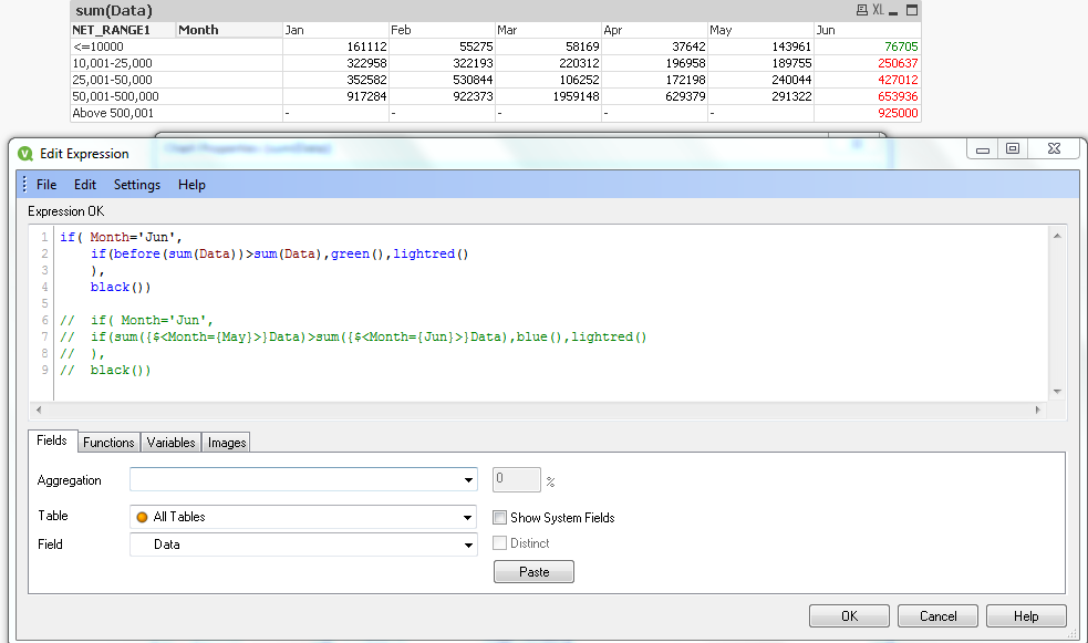
Please find the code and the screenshot.
I have used the data you provided.
if( Month='Jun',
if(before(sum(Data))>sum(Data),green(),lightred()
),
black())
Note : the Before would work only on a PIVOT table.
Regards,
Boo
Please mark correct answers if you find them.
- Mark as New
- Bookmark
- Subscribe
- Mute
- Subscribe to RSS Feed
- Permalink
- Report Inappropriate Content
Hi Upali,
In your Pivot Table, In the Expression window expand your Text Color box and enclose the below Definition.
=If(Sum({$<Month={'Jun'}>}Amount)<Sum({$<Month={'May'}>}Amount),Green(),Red())
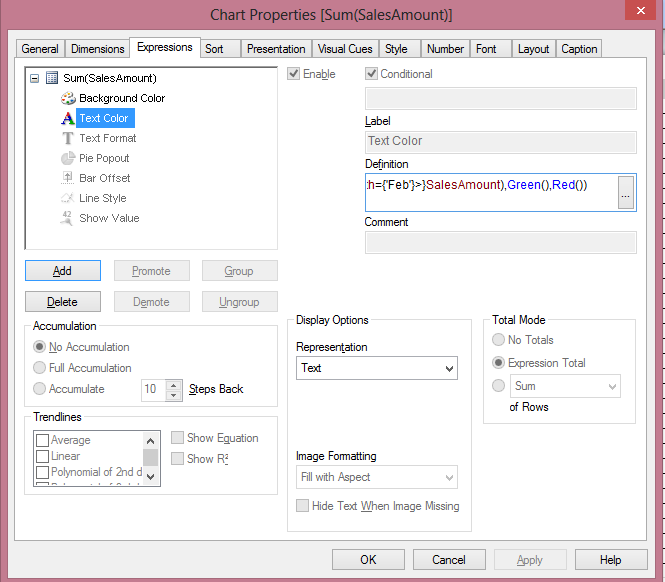
Many Thanks
Karthik
- Mark as New
- Bookmark
- Subscribe
- Mute
- Subscribe to RSS Feed
- Permalink
- Report Inappropriate Content
Perhaps This...!
vNetRange = Sum(NET_RANGE1)
=Aggr(If($(vNetRange) <= 10000, Green(),
If($(vNetRange) > 10001 and <=500000, Red(),
Black())),NET_RANGE1)
- Mark as New
- Bookmark
- Subscribe
- Mute
- Subscribe to RSS Feed
- Permalink
- Report Inappropriate Content