Unlock a world of possibilities! Login now and discover the exclusive benefits awaiting you.
- Qlik Community
- :
- All Forums
- :
- QlikView App Dev
- :
- Re: How to show color based on condition in EXCEL
- Subscribe to RSS Feed
- Mark Topic as New
- Mark Topic as Read
- Float this Topic for Current User
- Bookmark
- Subscribe
- Mute
- Printer Friendly Page
- Mark as New
- Bookmark
- Subscribe
- Mute
- Subscribe to RSS Feed
- Permalink
- Report Inappropriate Content
How to show color based on condition in EXCEL
Hi all,
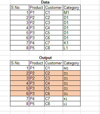
This is my source data.
I want highlight the cells in any color based on a condition in EXCEL file..
Condition:
For Category D1,Product P2,More than one Customer is there like C2,C3,C4,C5,C6.
Please advise.
Thanks in advance.
Sorry if my question is unrelated.
| S.No. | Product | Customer | Category |
| 1 | P1 | C1 | M1 |
| 2 | P2 | C2 | D1 |
| 3 | P2 | C3 | D1 |
| 4 | P3 | C4 | D1 |
| 5 | P3 | C5 | D1 |
| 6 | P3 | C6 | D1 |
| 7 | P4 | C7 | K1 |
| 8 | P5 | C8 | L1 |
Accepted Solutions
- Mark as New
- Bookmark
- Subscribe
- Mute
- Subscribe to RSS Feed
- Permalink
- Report Inappropriate Content
Hi Aretha,
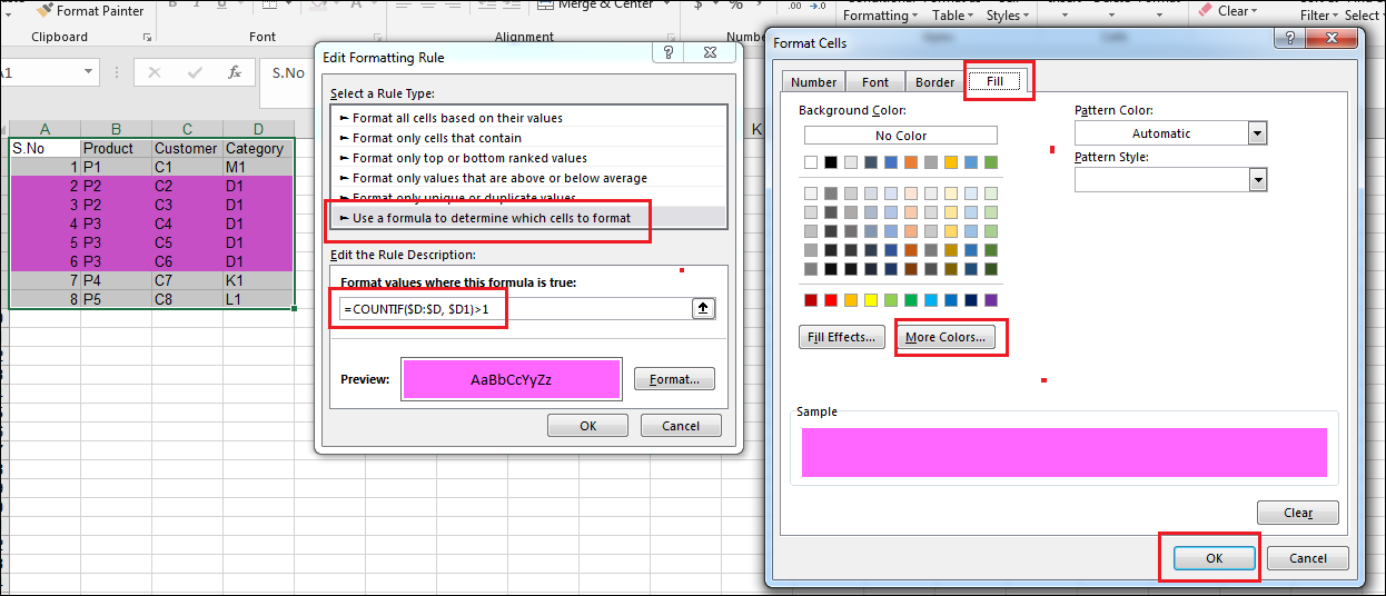
Formula: =COUNTIF($D:$D, $D1)>1
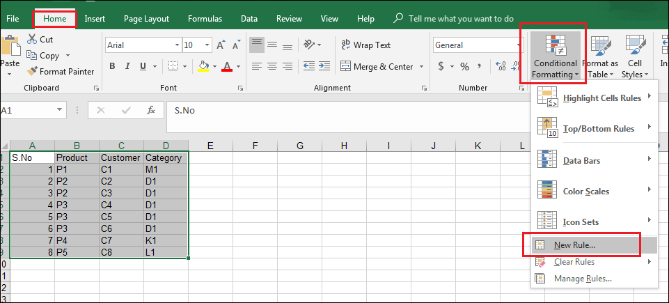
Step 1:
Goto Home -> Condition Formatting -> Select "New Rule"
Step 2:
Edit Formatting Rule -> Select "Use a Formula to determine which cells to format" -> Enter the above formula in "Format values where this formula is true" (Note that here the range is D column) -> Select "Format" button -> Use "Fill" tab to select the appropriate color (just play with other tabs and color options to explore more) -> press ok -> Apply -> Ok
- Mark as New
- Bookmark
- Subscribe
- Mute
- Subscribe to RSS Feed
- Permalink
- Report Inappropriate Content
Why would you like to ask the excel question in qlik community? Google for excel community and you would find many like: https://www.excelforum.com/
- Mark as New
- Bookmark
- Subscribe
- Mute
- Subscribe to RSS Feed
- Permalink
- Report Inappropriate Content
Apologies. I do not have access to that forum.
Please help me if possible.
- Mark as New
- Bookmark
- Subscribe
- Mute
- Subscribe to RSS Feed
- Permalink
- Report Inappropriate Content
Hi Aretha,
Formula: =COUNTIF($D:$D, $D1)>1
Step 1:
Goto Home -> Condition Formatting -> Select "New Rule"
Step 2:
Edit Formatting Rule -> Select "Use a Formula to determine which cells to format" -> Enter the above formula in "Format values where this formula is true" (Note that here the range is D column) -> Select "Format" button -> Use "Fill" tab to select the appropriate color (just play with other tabs and color options to explore more) -> press ok -> Apply -> Ok