Text color formatting in pivot table for Totals

[#1]

Hi,

     I have a pivot table with one of the dimension as journey status, which tracks down the journey for period of days. I have a requirement that I have to display the text in Red color for certain columns where the count is less than 1. To solve that, I have done the formatting in expression text color. But, the challenge that I am facing here is this coloring is being  applied for the total column ,which I am trying to eliminate.
I have tried using custom format cell but of no avail!

I am attaching the screenshot for reference!

[antoniotiman]

Hi,

use Dimensionality() like

=If(Dimensionality() > 0,If(Count(Field) < 0,Red()))

Regards,

Antonio

[Anonymous]

Try Visual Cues Option

[Anil_Babu_Samineni]

If(Dimensionality() = ColumnNo, Expression, Red())

[sky]

Hi,

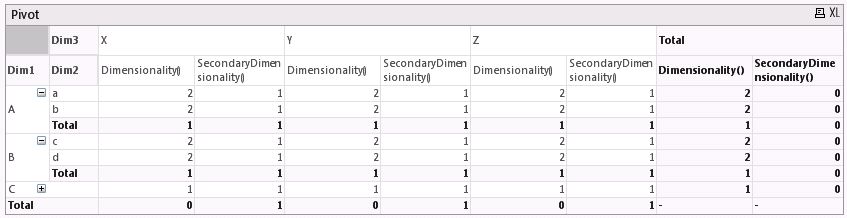
assuming that the day ranges are a dimension too, you´ll need the SecondaryDimensionality() expression.

As you can see in the screenshot, you just need to extend your expression with “if(SecondaryDimensionality() > 0, Red())”

 

[#6]

Hi,

   Thanks for the answer!

But, Dimensionality function isn't working for pivot table!

Can you temme if there is any other solution.

Thanks,

Navya

[antoniotiman · Accepted solution]

See attachment like Your screenshot

[#8]

It worked!

Thanks,

Navya