Customizing Pivot table partial Sum

[lionking15]

Hi Guys

Sno	Name	Sales
Q1	Jan	10
	Feb	20
	Mar	30
	Total	60
Q2	Apr	40
	May	50
	Jun	60
	Total	150

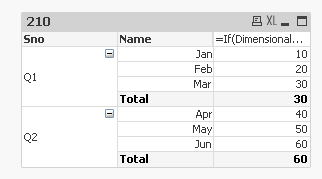
I want above pivot table as

Final Output

Sno	Name	Sales
Q1	Jan	10
	Feb	20
	Mar	30
	Total	30
Q2	Apr	40
	May	50
	jun	60
	Total	60

Total should be equal to max month of particular quarter.

[sunny_talwar · Accepted solution]

Try this expression:

=If(Dimensionality() = 1, FirstSortedValue(Aggr(Sum(Sales), Sno, Name), -Aggr(Name, Sno, Name)), Sum(Sales))

[vishsaggi]

May be try this in your expression:

= IF(Dimensionality() = 1,  Max(Sales), Sum(Sales))

[sunny_talwar]

What if the Max sales was associated with the month of Jan? I think the sample data might make us think that Max(Sales) will work, but in reality if we wish to pick the sales associated with Max month, we need to use FirstSortedValue here

[vishsaggi]

I got it now. You are right. We need firstsorted value.

[vinieme12]

or this

=If(Dimensionality() = 1,Sum({<Name = {"=Name = AGGR(Max(TOTAL <Sno> Name),Sno,Name)"}>}Sales) , Sum(Sales))